Project 5 - Diffusion Models

Approach

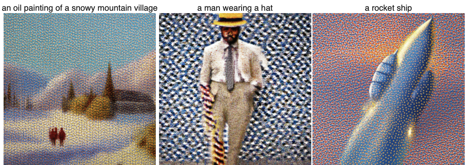
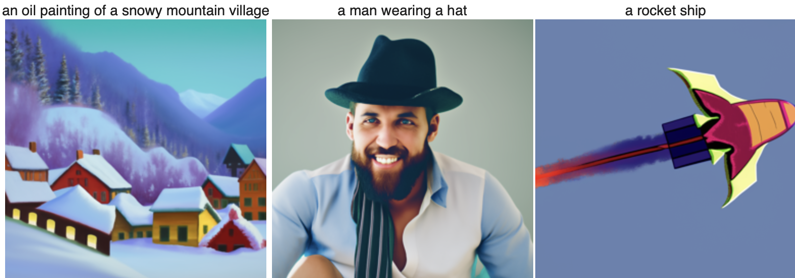
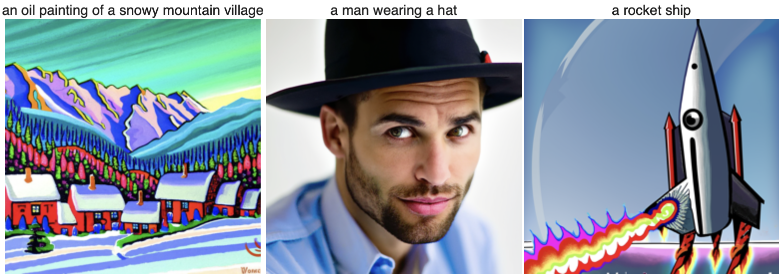
I ran the code for num_inference_steps = 5, 10, 100. The quality of the images, especially for the man, improved with more inference steps.

Results

Approach

Starting from a clean image, noise was progressively added at each timestep until reaching pure noise at T = 1000. Using the model, I reversed this process by predicting and removing noise step-by-step to reconstruct the original image. Noise levels were controlled by DeepFloyd’s pre-set coefficients, alphas_cumprod. The sample image was resized to 64 × 64, scaled to [-1, 1], and prepared as input for the denoising process. The random seed I am using is 3141592.

Results

Approach

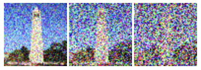
I implemented the forward process to simulate noise addition to a clean image at varying levels. Given a clean image x_0, the forward process generates a noisy image x_t at timestep t by sampling from a Gaussian distribution with mean sqrt(alphas_cumprod[t]) * x_0 and variance (1 - alphas_cumprod[t]). Using the function forward, I applied this process to the test image for noise levels t = 250, 500, and 750, resulting in progressively noisier images as expected.

Results

Approach

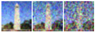
Denoising techniques was applied to the noisy images from timesteps 250, 500, and 750 using Gaussian blur filtering. Each noisy image was processed with torchvision.transforms.functional.gaussian_blur to attempt noise reduction. The results were displayed side by side to compare the effectiveness of Gaussian denoising on each image. Achieving significant noise reduction proved challenging due to the limitations of classical filtering methods with high-noise images.

Results

Approach

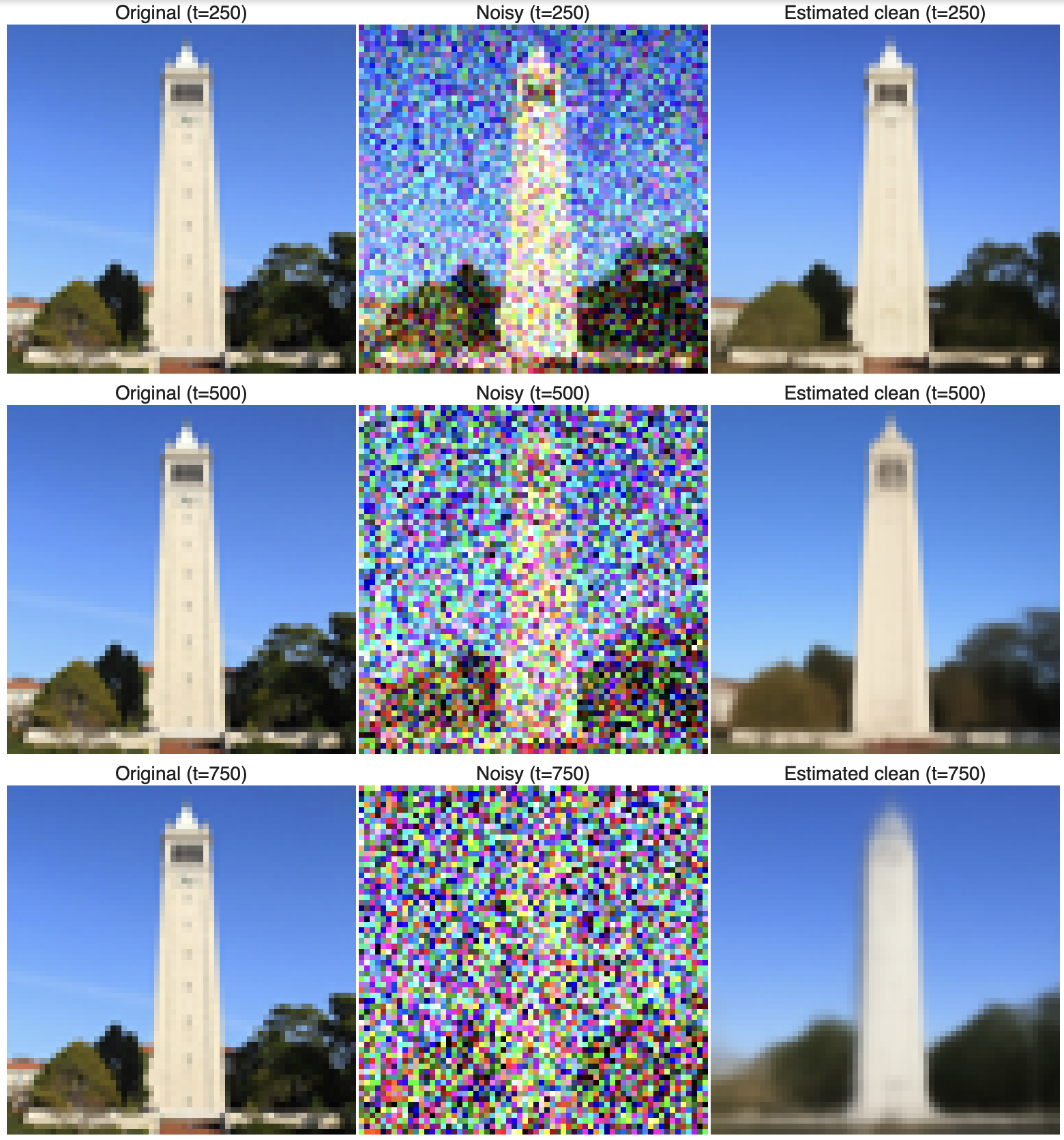
Here, I used a pretrained UNet, to perform one-step denoising on noisy images. This UNet was trained on a vast dataset of image pairs (x_0, x_t) and can estimate the noise present in a noisy image x_t when given a specific timestep t. By estimating the noise, I was able to subtract it (while applying the necessary scaling, as per equation 2) to recover an approximation of the original image x_0. This process was applied to images with noise levels t = [250, 500, 750], and the results were visualized side-by-side, showing the original, noisy, and estimated denoised images.

Results

Approach

Next, I implemented iterative denoising by starting with a noisy image at t = 990, and I progressively reduced noise at strided timesteps, which interpolates between signal and noise. Key parameters like alpha, beta, and alphas_cumprod were computed at each step, with variance added via the add_variance function to mimic training conditions. Intermediate results every 5 steps showed gradual noise reduction.

Results

Approach

A diffusion model was used to generate images from scratch by denoising pure random noise. The process involved creating random noise tensors using torch.randn and then denoising the tensors with the iterative_denoise function. We applied a prompt embedding for "a high quality photo" to guide the generation process and repeated this five times to produce unique images.

Results

Approach

I used Classifier-Free Guidance (CFG) to enhance image quality by combining conditional and unconditional noise estimates with a scaling factor, γ, set to 7. This involved implementing the iterative_denoise_cfg function, which denoises images using both a prompt embedding for "a high quality photo" and an empty prompt embedding for unconditional guidance. The UNet model was run twice at each timestep to compute the conditional and unconditional noise estimates, which were then combined using the CFG formula. I did this five times, to generate images with significantly improved quality compared to the previous section.

Results

Approach

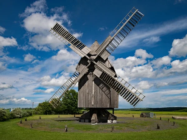
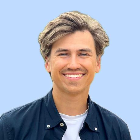
I used the SDEdit algorithm to refine noisy images back to natural-looking ones. Starting with the test image, I added noise and denoised it using the iterative_denoise_cfg function with starting indices [1, 3, 5, 7, 10, 20]. The process was guided by the prompt "a high quality photo" and a CFG scale of 7. I also repeated this on two other test images to show how the method works for different inputs. The model seems to have a bias agains women, as the generated images mostly contain women, even though the original image has nothing to do with it.

Results

Approach

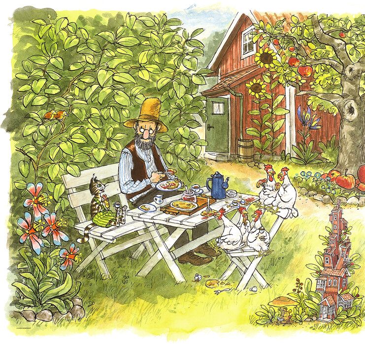
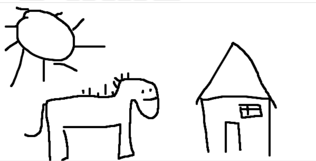
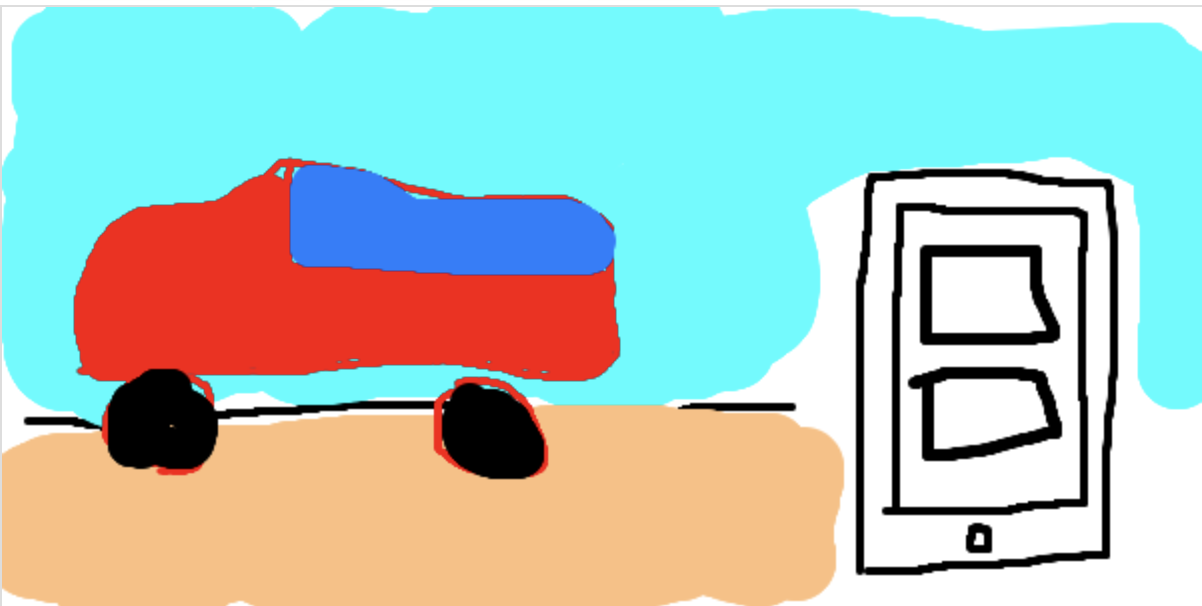
I experimented with editing non-realistic images, including one downloaded from the web and two hand-drawn images. Using the iterative_denoise_cfg function, I applied the same noise levels ([1, 3, 5, 7, 10, 20]) to project these images onto the natural image manifold. The preprocessing steps ensured the input images fit the model's requirements, with resizing and normalization. Results demonstrate how effectively the algorithm transforms diverse inputs into photorealistic images.

Results - Web Image

Results - Hand drawn image

Approach

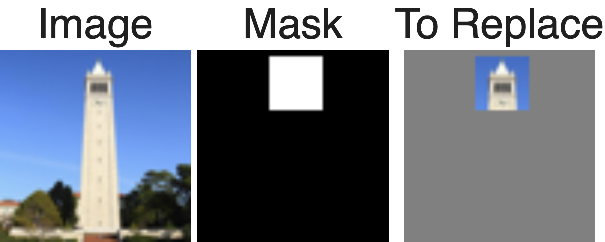
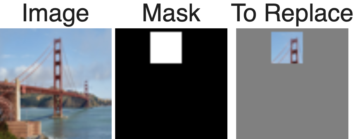
This function uses a binary mask to retain the original image content in unmasked areas while applying iterative denoising to generate new content in masked areas. I created a mask for the Campanile test image and inpainted the top of the tower. Additionally, I edited two custom images using unique masks for creative inpainting tasks. The results demonstrate the ability to seamlessly blend original and generated content.

Result - Campanile

Results - Custom images

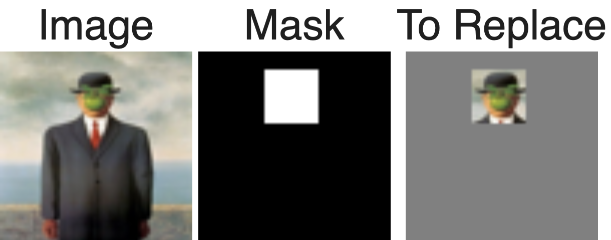
Perfect! I have always wondered what the face behind the apple looks like. Now we all know.

Approach

In this step, I used the text prompt "a rocket ship" to guide how an image evolves during denoising. Starting with varying noise levels [1, 3, 5, 7, 10, 20], the process blends the original image with rocket-themed elements. I also applied this to two of my own images, showing how text prompts can creatively transform visuals!

Results

Results - Custom Images

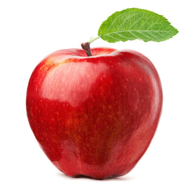
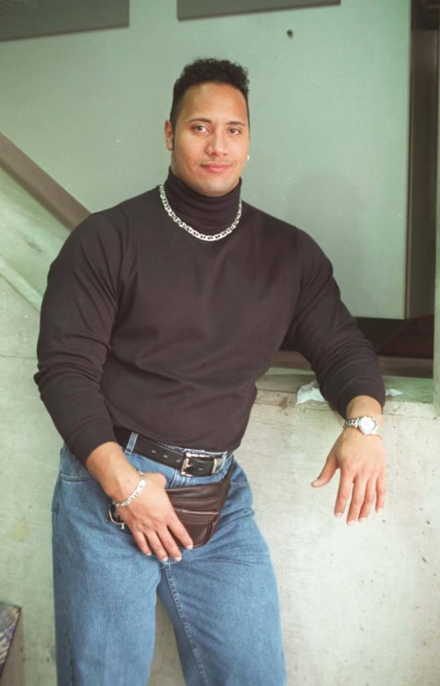
I wanted to test the algorithm to see how it behaves on images which does not resemble rocket ships at all. On a low noise level it creates rocket ships, but the higher the noise, the more it resembles the original image.

Approach

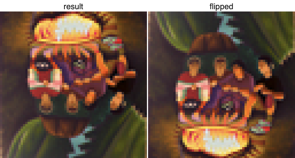
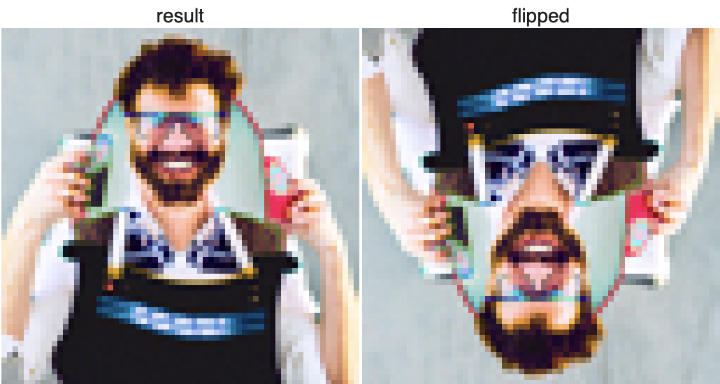
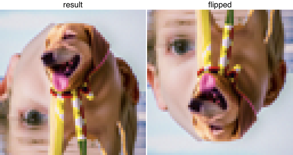
The Visual Anagrams technique creates an optical illusion where an image of "an oil painting of an old man" turns into "an oil painting of people around a campfire" when flipped upside down. By denoising the image with two different prompts—one for the original and one for the flipped version—and averaging the noise estimates, we get this effect. Here’s an example where flipping the image reveals a completely different scene.

Results

Approach

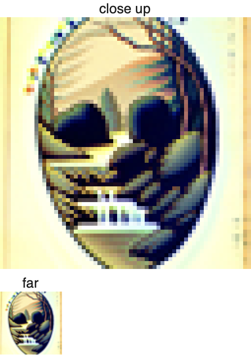
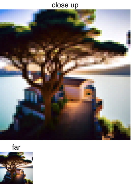
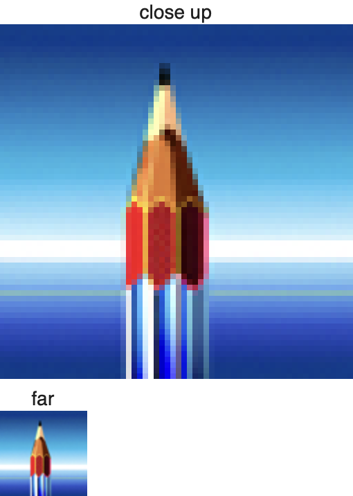
The Hybrid Images technique combines low-frequency details from one image and high-frequency details from another using a diffusion model. By generating separate noise estimates for each image with different text prompts and applying low-pass and high-pass filters, we blend the two to create an image that looks like one object from afar and another up close.

Results

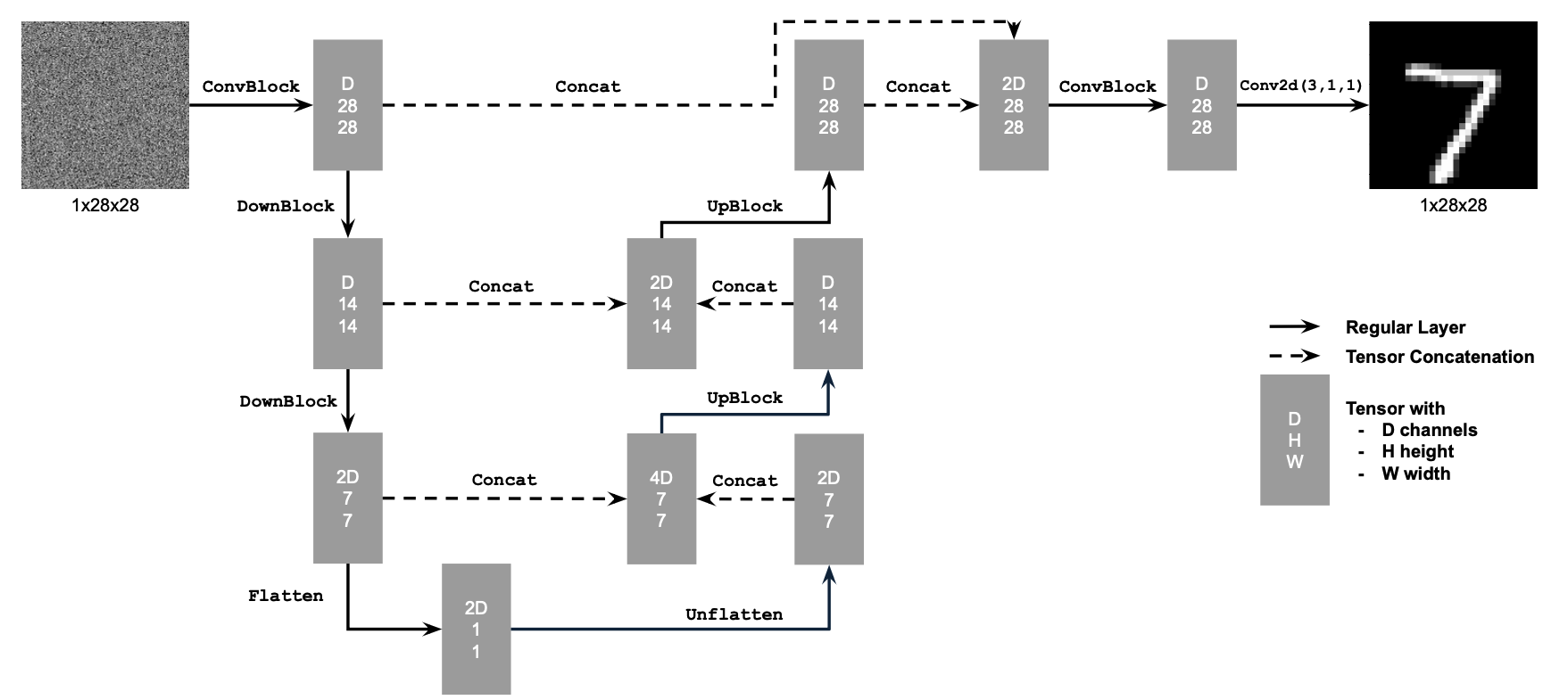
I implemented U-Net which takes a noisy image as input and predicts the noise from the original image. It consists of down and upsampling blcok with skip connections. This captures both global and local features. The UNet structure is good for image-to-image task, for example denoising.

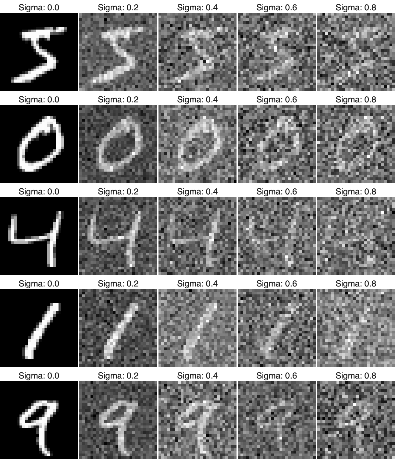
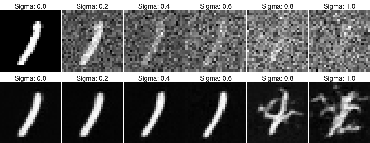
Below are the results from visualizing the effect of sigma=0.5 on adding noise to the image, so the model only sees one sigma. The loss quickly reduces and the train and test loss intersects at around 0.009.

For training, I used the image class pairs from MNIST dataset. I used batch_size = 256, num_epochs = 5, sigma = 0.5, and the Adam optimizer with a learning rate of 0.0001.

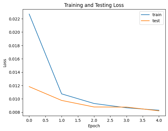
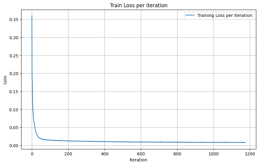
Below, the results from the training can be seen, where the performacce between the results from 1 epoch and 5 epochs can be seen. The model is much better at denoising after 5 epochs.

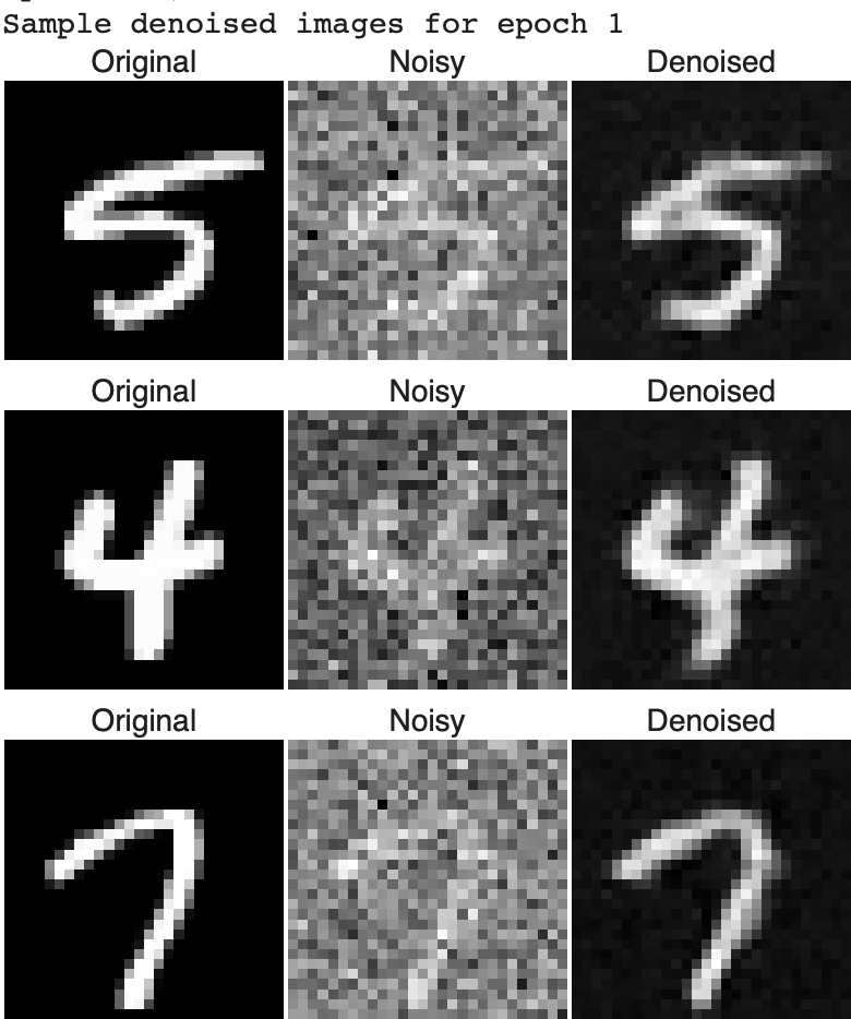
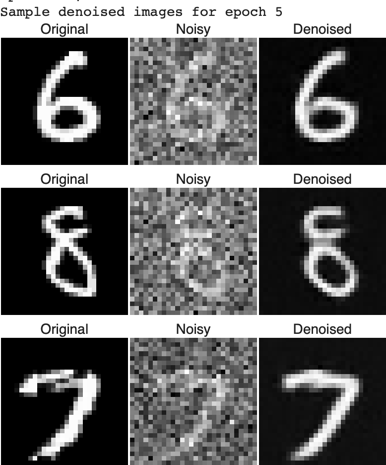
It is interesting to observe its performance with different sigma values, representing higher and lower noise levels than those used during training. The image below illustrates this performance.

In the previous section, the UNet model was designed to predict the clean image directly. In this section, I modify the approach to predict the noise ϵ that was added to the image. This adjustment enables us to begin with pure noise ϵ ∼ N(0, I) and progressively denoise it to produce a realistic image x.

Combination of Time and Class Conditioning

We condition the UNet on both the timestep t and the digit class simultaneously. Using the equation: xt = √ᾱtx0 + √(1−ᾱt)ϵ, where ϵ∼N(0,1), we generate a noisy image xt from x0 for a timestep t∈{0,1,…,T}. At t=0, xt is the original clean image, and at t=T, xt is entirely noise. For intermediate values of t, xt is a blend of the clean image and noise. We set T = 400 due to the simplicity of our dataset. Time conditioning is incorporated using fully connected layers to embed t into the UNet, and class conditioning uses one-hot vectors and additional fully connected layers to embed the class vector. Below is the updated UNet architecture, which includes both time and class conditioning, as well as the new training algorithm used.

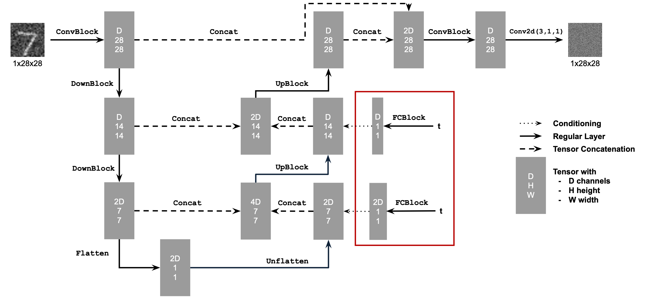
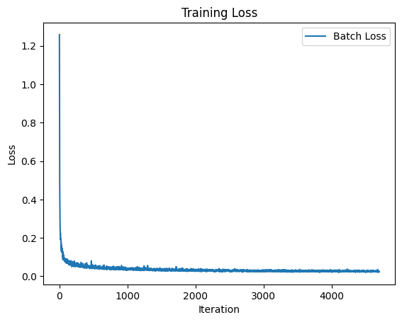
During training, noisy images, xt, are created for random timesteps, and their one-hot class vectors are computed. The UNet is then trained to predict ϵ. By incorporating class conditioning, we achieve better control over the generated images, while time conditioning facilitates iterative denoising. The results below, after the twentieth epoch, demonstrate that the model performs exceptionally well, producing accurate and detailed numbers. Below is the results from the time and class conditional UNet.

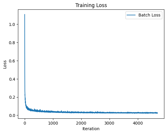
We can compare this to the Time Conditioned UNet which has no classes. The results can be seen below. As seen, the numbers are not as good without the classifier free guidance.