Project 4 - (Auto)Stitching Photo Mosaics

Filip Malm-Bägén

Part A - Introduction

This first part of the project goes through image warping and mosaicing. The goal is to create a panorama image from multiple images.

Shoot the Pictures

Approach

I took a lot of different pictures. The important things which I had in mind were that I must rotate the camera strictly around the optical center of the camera. In the beginning, I was careless about this, which resulted in a lot of problems. I also made sure to photograph scenes far away from the camera. This is important because the parallax effect is less significant when the objects are far away from the camera. I also made sure to have a lot of overlap between the images. This is important because the more overlap there is, the more information there is to stitch the images together.

Recover Homographies

Approach

I got the correspondig points using the same tool as used in project 3 to label the points of the two images. After getting the correspondig points, I used SVD to get the homography matrix. Once I had the points, I set up a system of linear equations. For each pair of corresponding points, I derived two equations, resulting in a system with as many equations as twice the number of points. To solve for the homography matrix, I used Singular Value Decomposition (SVD). This method allowed me to solve the system in a least-squares manner, which is more stable when dealing with more than the minimum four points. The final step involved reshaping the solution into a 3x3 matrix and normalizing it so that the lower-right corner was 1. This homography matrix is what I used to warp one image onto the other, aligning them for blending.

Warp the Images

Approach

To warp the image using the homography matrix, I transformed the corners of the original image represented as homogeneous coordinates by multiplying them with the homography matrix H. After normalizing the resulting coordinates, I determined the new bounds for the warped image. Next, I created a meshgrid for the output image's coordinates and mapped them back to the input image using the inverse homography matrix, H_inv. This reverse mapping allowed me to retrieve pixel values from the original image. For each channel, I employed the griddata function for linear interpolation, filling in pixel values smoothly across the warped image. Finally, the function returned the warped image, facilitating accurate alignment in subsequent steps, such as image stitching or blending.

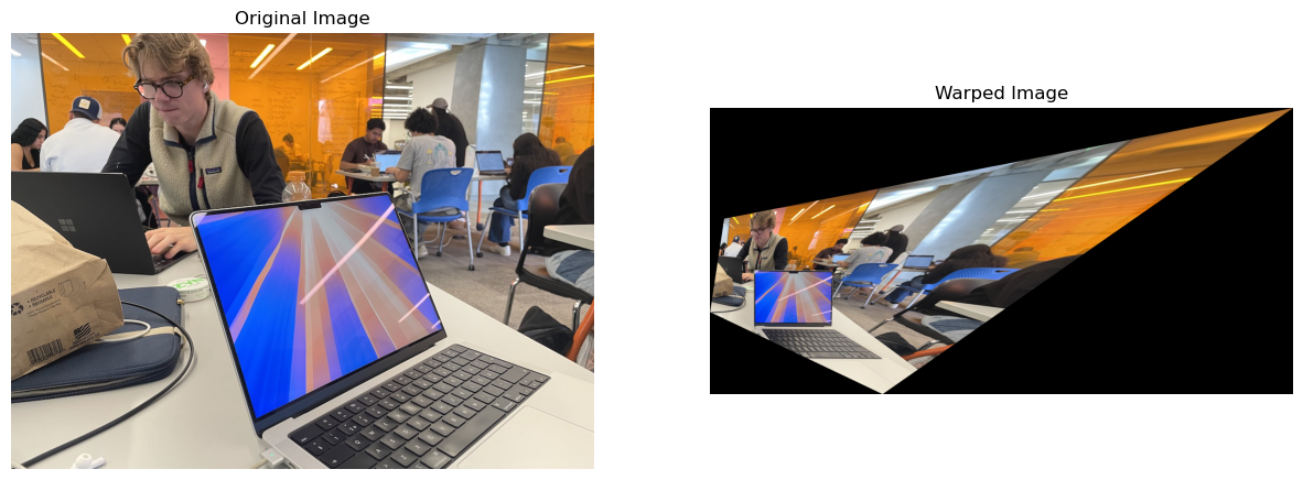
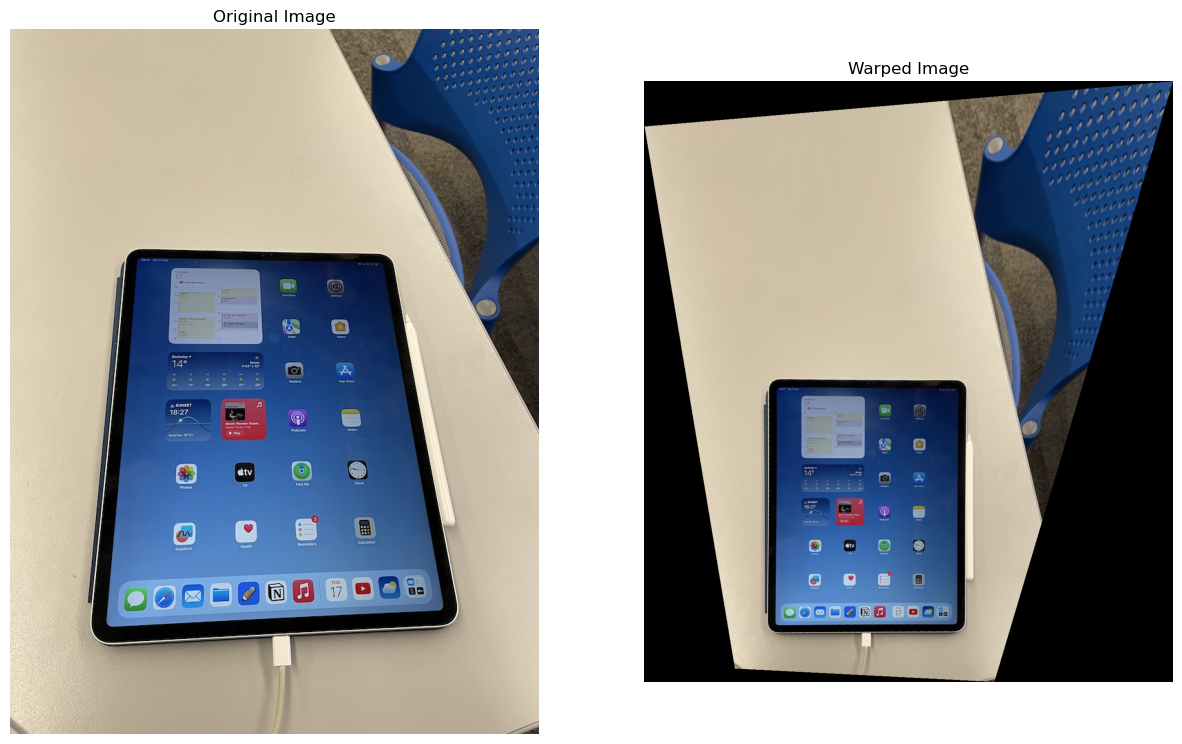
Image Rectification

Blend the images into a mosaic

Approach

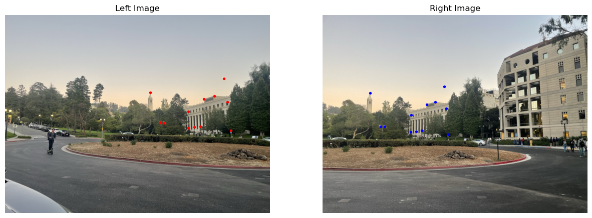
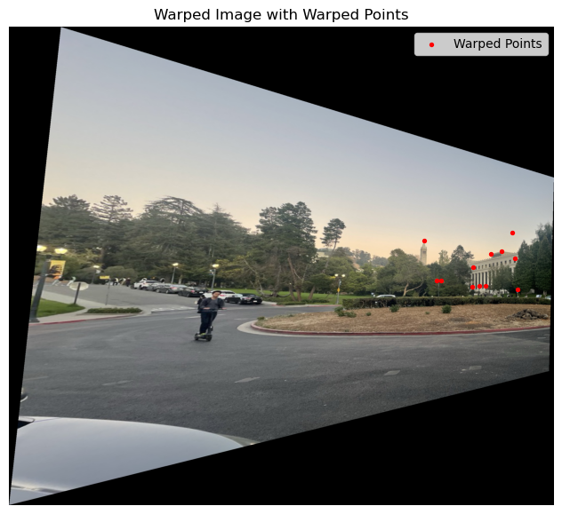
I began by loading two new images, panorama_left and panorama_right, along with their corresponding points from a JSON file. I visualized these images alongside the marked points for reference. Using the function computeH, I calculated the homography matrix H2 to warp the left image into the perspective of the right image. The warped points of the left image were computed using the warpPoints function, which adjusted their coordinates based on the new position on the warped image. 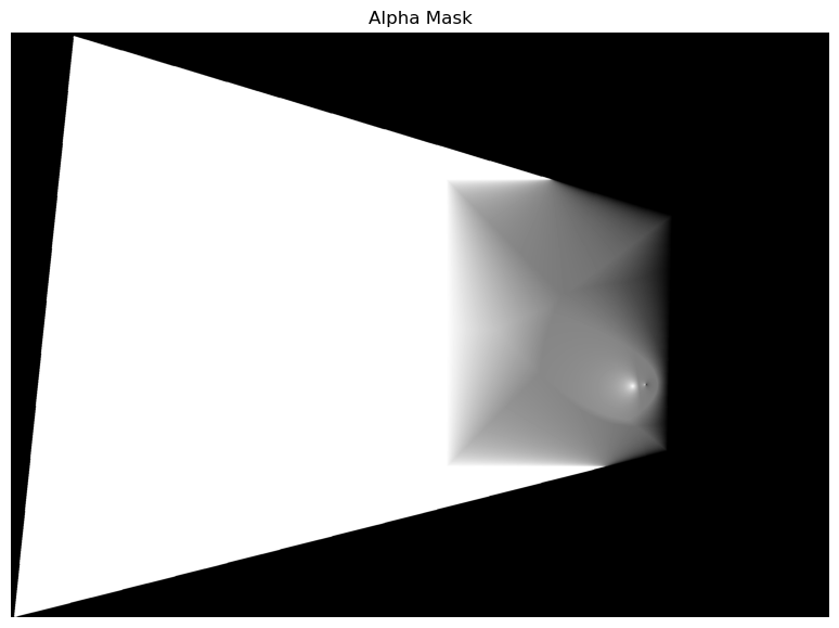Next, I created a blending mask to seamlessly merge the two images. This involved calculating the distance transform of both images and generating an alpha mask to facilitate blending. 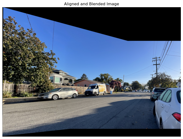I also implemented the align_and_blend_images function, which calculated the necessary transformations to align and blend the warped left image with the right image accurately. Finally, the resultant aligned and blended image was displayed, showcasing the effectiveness of the mosaicing process.

Results

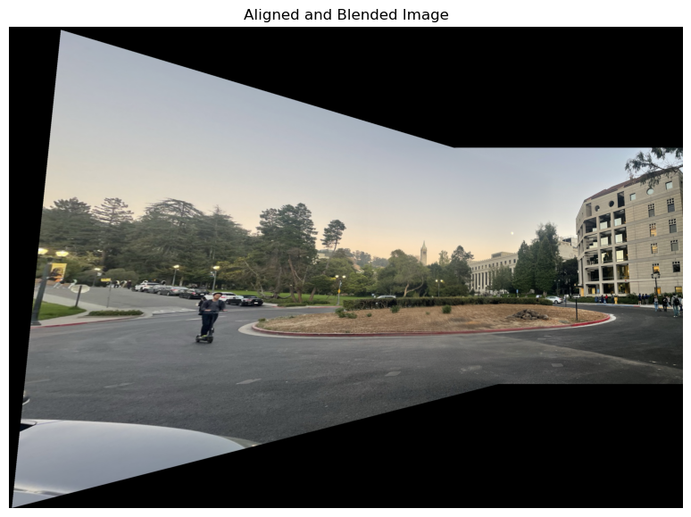
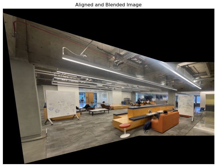
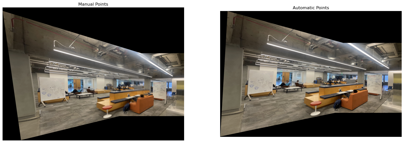
Finally, I wanted to test the limits of the algorithm and took two images over Moffitt Library with a thin overlap (not even 40%, which was the recomended minimum). The result was not perfect, but it was still quite impressive. The algorithm managed to stitch the images together, but the seam is very blurry and not very well aligned. This can also be due to careless photography, or careless placement of the corresponding points. The result is still quite impressive, considering the lack of overlap.

Part B - Introduction

This second part of the project goes through the process of stiching images together into mosaics using corresponding points. The points are automaticaly identified, filtered and matched. The goal is to automaticaly create a panorama image from multiple images.

Interest Point Detector

Approach

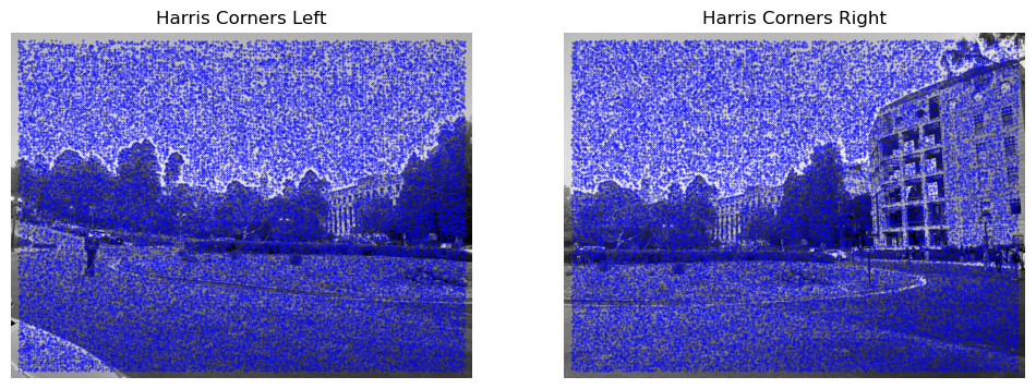
In the first step, I used the Harris corner detection algorithm to identify interest points. The images were converted to grayscale, and corners were detected using get_harris_corners(). The function returned the corner strength map h and corner coordinates, which were then plotted on the grayscale images. The detected corners were visualized as blue points, showing the key points of interest for further image stitching.

Result

Adaptive Non-Maximal Suppression

Approach

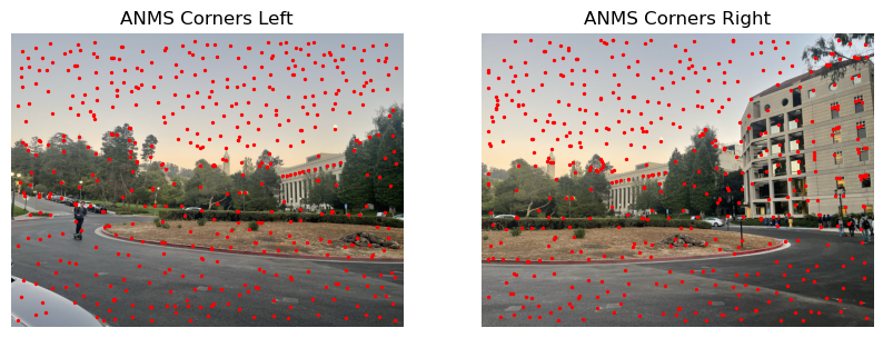
Next, I implemented Adaptive Non-Maximal Suppression (ANMS) to select the strongest and most spatially distributed corners. The Harris scores were used to compare corners, and pairwise distances were computed with dist2(). Based on these distances and corner strengths, a suppression process determined the minimum radius for each point. The top corners were then selected and visualized as red points on the images.

Result

Feature Descriptor Extraction

Approach

For each corner detected through ANMS, I extracted feature descriptors by sampling an axis-aligned 8x8 patch from a larger 40x40 window around each point. The larger window was first blurred using a Gaussian filter to ensure smoothness and reduce aliasing. Each patch was sampled with a spacing of 5 pixels and bias/gain-normalized by subtracting the mean and dividing by the standard deviation of the pixel values. Descriptors for each corner were created by concatenating the normalized patches from all three color channels into a single vector, forming a feature descriptor for each point.

Result

Feature Matching

Approach

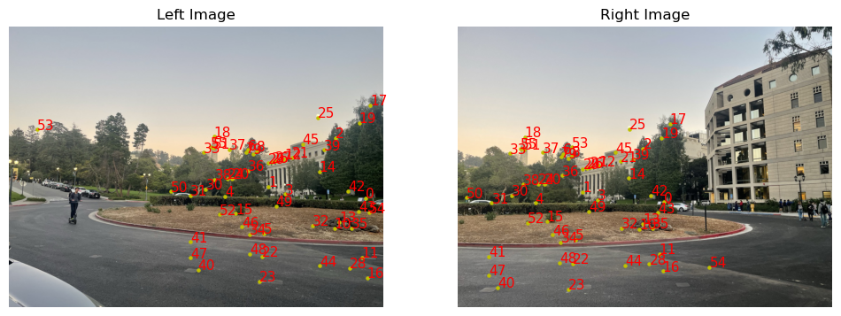
To match feature descriptors between the two images, I implemented a feature matching algorithm based on Lowe's ratio test. For each feature in the first image, I calculated the distances to all feature descriptors in the second image using Euclidean distance. The two nearest neighbors were identified, and Lowe's ratio test was applied to ensure that the nearest neighbor is sufficiently better than the second. If the distance to the nearest neighbor was less than a specified threshold times the distance to the second, the match was retained. This process ensured robust feature matching and prevented incorrect matches due to ambiguous descriptors. One-to-one matching was enforced by keeping track of already matched points in the second image.

Result

4-Point RANSAC

Approach

Finally, I implemented the RANSAC algorithm to find the best homography matrix for aligning two sets of points. Given sets of corresponding coordinates, coords_1 and coords_2, and a list of matched pairs matches, the function ransac iterates a specified number of times to find the optimal set of inliers. In each iteration, four random points from each set are sampled to compute a homography matrix H_temp using computeH. This homography is then applied to all points in pts1 using the warp_points_ransac function, which converts points into homogeneous coordinates, applies the transformation matrix, and scales the result to get the transformed points. The transformed points are compared to their target points from pts2 by calculating the Euclidean distance, with any points within the threshold distance considered inliers. If the count of inliers exceeds the current maximum, the inlier set is updated to best_inliers. After iterating, a final homography matrix final_H is calculated using all the points in best_inliers, representing the best transformation for the image alignment.

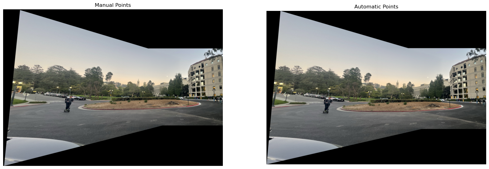
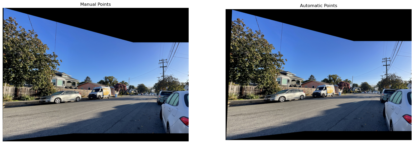
After implementing the RANSAC algorithm, I warped the image and blended the images into mosaic using the same code as in part A. The result was a a panorama image from multiple images, similar to the result from part A, but without any manual work. The result is quite impresive, and the coolest thing I learned in this project was how efficient the algorithm is, and that I now know how to stitch images.

Result

Interestringly, the image used on previous exercise to test the limit of my algorithm now works great. Even though the overlap is less than 40%, my new implementation perfectly aligns the images, and gives no blurry edges (which the previous image had).